
In this blog we look at a method to estimate where to prioritise your SEO resources, estimating which keywords will give the greatest increase in revenue if you could improve their Google rank.
Overview
Thanks to Vincent at data-seo.com who proof read and corrected some errors in the first draft
Data comes from Google Search Console and Google Analytics.
Search Console is used to provide the keywords in these days post (not provided). We then link the two data sets by using the URLs as a key, and estimate how much each keyword made in revenue by splitting them in the same proportion as the traffic they have sent to the page.
This approach assumes each keyword converts at the same rate once on the page, and will work better with some websites more than others - the best results I have seen are those websites with a lot of content on seperate URLs, such that they capture long-tail queries. This is because the amount of keywords per URL is small, but with enough volume to make the estimates trustworthy.
We also try to incorporate magins of error in the results. This avoids situations where one click on position 40 gets a massive weighting in potential revenue, which in reality could have been a freak event.
Summary
The method produced a targeted keyword list of 226 from an original seed list of ~21,000. The top 30 revenue targets are shown in the plot below:
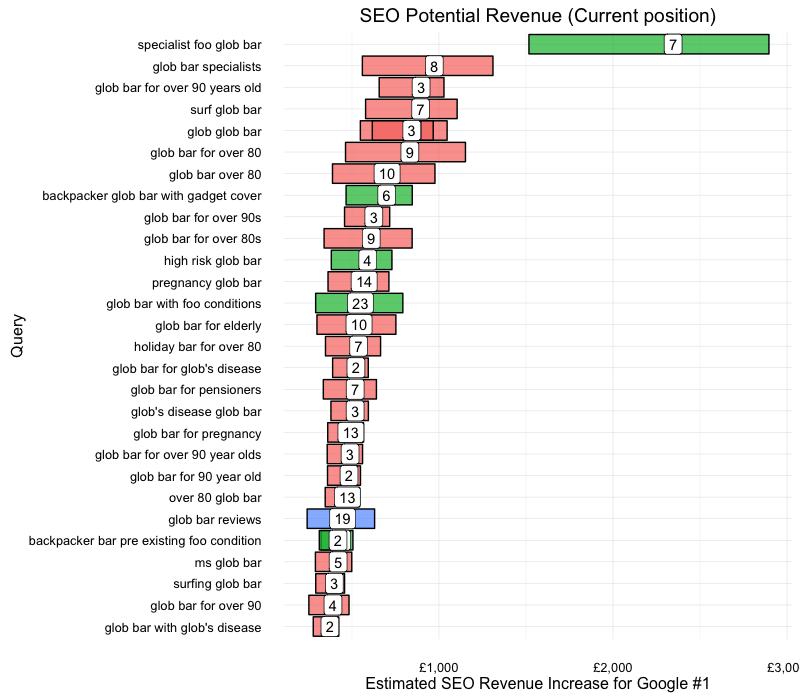
Read below on how the plot was generated and what the figures mean.
Getting the data
Google Analytics recently provided more integration between the Search Console imports and the web session data, of which Daniel Waisberg has an excellent walk-through, which could mean you can skip the first part of this script.
However, there are circumstances where the integration won’t work, such as when the URLs in Google Analytics are a different format to Search Console - with the below script you have control on how to link the URLs, by formatting them to look the same.
Data is provided via my searchConsoleR and googleAnalyticsR R packages.
library(searchConsoleR)
library(googleAnalyticsR)

## authentication with both GA and SC
options(googleAuthR.scopes.selected =
  c("https://www.googleapis.com/auth/webmasters",
    "https://www.googleapis.com/auth/analytics",
    "https://www.googleapis.com/auth/analytics.readonly"))

googleAuthR::gar_auth()

## replace with your GA ID
ga_id <- 1111111

## date range to fetch
start <- as.character(Sys.Date() - 93)
end <- "2016-06-01"

## Using new GA v4 API
## GAv4 filters
google_seo <-
  filter_clause_ga4(list(dim_filter("medium",
                                     "EXACT",
                                     "organic"),
                          dim_filter("source",
                                     "EXACT",
                                     "google")),
                     operator = "AND")

## Getting the GA data
gadata <-
  google_analytics_4(ga_id,
                     date_range = c(start,end),
                     metrics = c("sessions",
                                 "transactions",
                                 "transactionRevenue"),
                     dimensions = c("landingPagePath"),
                     dim_filters = google_seo,
                     order = order_type("transactions",
                                        sort_order = "DESC",
                                        orderType = "VALUE"),
                     max = 20000)

## Getting the Search Console data
## The development version >0.2.0.9000 lets you get more than 5000 rows
scdata <- search_analytics("http://www.example.co.uk",
                           startDate = start, endDate = end,
                           dimensions = c("page","query"),
                           rowLimit = 20000)
Transforming the data
First we change the Search Console URLs into the same format as Google Analytics. In this example, the hostname is appended to the GA URLs already (a reason why the native support won’t work), but you may also need to append the hostname to the GA URLs via paste0("www.yourdomain.com", gadata$page).
We also get the search page result (e.g. Page 1 = 1-10, Page 2 = 11-20) as it may be useful.
For the split of revenue later, the last call calculates the % of clicks going to each URL.
Search Console data transformation
library(dplyr)

## get urls in same format

## this will differ from website to website,
## but in most cases you will need to add the domain to the GA urls:
## gadata$page <- paste0("www.yourdomain.com", gadata$landingPagePath)
## gadata has urls www.example.com/pagePath
## scdata has urls in http://www.example.com/pagePath
scdata$page2 <- gsub("http://","", scdata$page)

## get SERP
scdata$serp <- cut(scdata$position,
                   breaks = seq(1, 100, 10),
                   labels = as.character(1:9),
                   include.lowest = TRUE,
                   ordered_result = TRUE)

## % of SEO traffic to each page per keyword
scdata <- scdata %>%
  group_by(page2) %>%
  mutate(clickP = clicks / sum(clicks)) %>%
  ungroup()
Merging with Google Analytics
Now we merge the data, and calculate the estimates of revenue, transactions and sessions.
Why estimate sessions when we already have them? This is how we assess how accurate this approach is - if the clicks is roughly the same as the estimated sessions, we can go further.
The accuracy metric is assessed as the ratio between the estiamted sessions and the clicks, minus 1. This will be 0 when 100% accuracy, and then the further away from 0 the figure is the less we trust the results.
We also round the avergae position to the nearest whole number.
library(dplyr)

## join data on page
joined_data <- gadata %>%
  left_join(scdata, by = c(landingPagePath = "page2")) %>%
  mutate(transactionsEst = clickP*transactions,
         revenueEst = clickP*transactionRevenue,
         sessionEst = clickP*sessions,
         accuracyEst = ((sessionEst / clicks) - 1),
         positionRound = round(position))

## we only want clicks over 0, and get rid of a few columns.
tidy_data <- joined_data %>%
  filter(clicks > 0) %>%
  select(-page, -sessions, -transactions, -transactionRevenue)
Is it reliable?
A histogram of the accuracy estimate shows we consistently over estimate but the clicks and estimated sessions are within a magnitude:
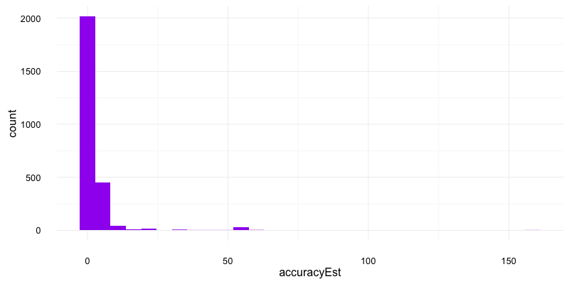
Most of the session estimates were intrestingly around 1.3 times more than the clicks. This may be because Search Console clicks act more like Google SEO users, but any other ideas please say in comments!
From above I discarded all rows with an accuracy > 10 as unreliable, although you may want to be stricter in your criteria. All figures are to be taken with a pinch of salt with this many assumptions, but if the relative performance looked ok then I feel there is still enough to get some action from the data.
Creating the SEO forecasts
We now use the data to create a click curve table, with estimates on the CTR for each position, and the confidence in those results.
I first attempted some models on making predictions of click curves for a website, but didn’t find any general satisifactory regressions.
The diagram below uses a weighted loess within ggplot2 which is good to show trend but not for making predictions.
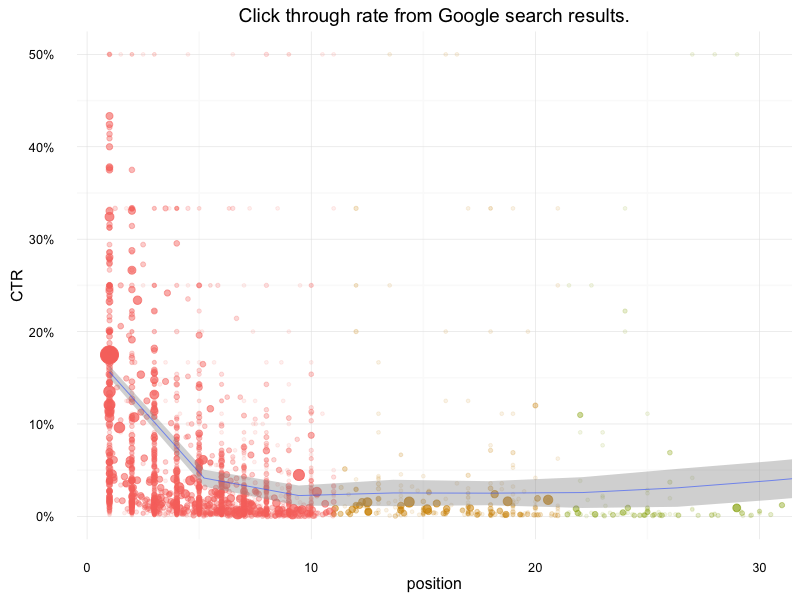
A click curve to use
However, 99% of the time we will only be concerned with the top 10, so it wasn’t too taxing to calculate the click through rates per website based on the data they had:
library(dplyr)

click_curve <- tidy_data %>%
  group_by(positionRound) %>%
  summarise(CTRmean = sum(clicks) / sum(impressions),
            n = n(),
            click.sum = sum(clicks),
            impressions.sum = sum(impressions),
            sd = sd(ctr),
            E = poisson.test(click.sum)$conf.int[2] / poisson.test(impressions.sum)$conf.int[1],
            lower = CTRmean - E/2,
            upper = CTRmean + E/2) %>% ungroup()

## add % increase to position 1
## could also include other positions
click_curve <- click_curve %>%
  mutate(CTR1 = CTRmean[1] / CTRmean,
         CTR1.upper = upper[1] / upper,
         CTR1.lower = lower[1] / lower)
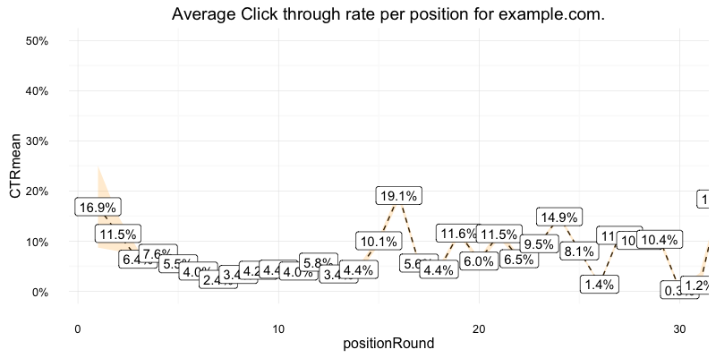
These CTR rates are then used to predict how much more traffic/revenue etc. a keyword could get if they moved up to position 1.
How valuable is a keyword if position 1?
Once happy with the click curve, we now apply it to the original data, and work out estimates on SEO revenue for each keyword if they were at position 1.
I trust results more if they have had more than 10 clicks, and the accuracy estimate figure is within 10 of 0. I would play around with this limits a little yourself to get something you can work with.
library(dplyr)
## combine with data

predict_click <- tidy_data1 %>%
  mutate(positionRound = round(position)) %>%
  left_join(click_curve, by=c(positionRound = "positionRound")) %>%
  mutate(revenueEst1 = revenueEst * CTR1,
         transEst1 = transactionsEst * CTR1,
         clickEst1 = clicks * CTR1,
         sessionsEst1 = sessionEst * CTR1,
         revenueEst1.lower = revenueEst * CTR1.lower,
         revenueEst1.upper = revenueEst * CTR1.upper,
         revenueEst1.change = revenueEst1 - revenueEst)

estimates <- predict_click %>%
  select(landingPagePath, query, clicks, impressions,
         ctr, position, serp, revenueEst, revenueEst1,
         revenueEst1.change, revenueEst1.lower, revenueEst1.upper,
         accuracyEst) %>%
  arrange(desc(revenueEst1)) %>%
  dplyr::filter(abs(accuracyEst) < 10,
                revenueEst1.change > 0,
                clicks > 10)
estimates now in this example holds 226 rows sorted in order or how much revenue they are to make if position #1 in Google. This is from an original keyword list of 21437, which is at least a way to narrow down to important keywords.
Plotting the data
All that remains to to present the data: limiting the keywords to the top 30 lets you present like below.
The bars show the range of the estimate, as you can see its quite wide but lets you be more realistic in your expectations.
The number in the middle of the bar is the current position, with the revenue at the x axis and keyword on the y.
ggplot2 code
To create the plots in this post, please see the ggplot2 code below. Feel free to modify for your own needs:
library(ggplot2)

## CTR per position
ctr_plot <- ggplot(tidy_data, aes(x = position,
                                  y = ctr
                                  ))
ctr_plot <- ctr_plot + theme_minimal()
ctr_plot <- ctr_plot + coord_cartesian(xlim = c(1,30),
                                       ylim = c(0, 0.5))
ctr_plot <- ctr_plot + geom_point(aes(alpha = log(clicks),
                                      color = serp,
                                      size = clicks))
ctr_plot <- ctr_plot + geom_smooth(aes(weight = clicks),
                                   size = 0.2)
ctr_plot + scale_y_continuous(labels = scales::percent)
ctr_plot

hh <- ggplot(click_curve, aes(positionRound, CTRmean))
hh <- hh + theme_minimal()
hh <- hh + geom_line(linetype = 2) + coord_cartesian(xlim = c(1, 30),
                                                     ylim = c(0,0.5))
hh <- hh + geom_ribbon(aes(positionRound, ymin = lower, ymax = upper),
                       alpha = 0.2,
                       fill = "orange")
hh <- hh + scale_y_continuous(labels = scales::percent)
hh <- hh + geom_point()
hh <- hh + geom_label(aes(label = scales::percent(CTRmean)))
hh


est_plot <- ggplot(estimates[1:30,],
                   aes(reorder(query, revenueEst1),
                       revenueEst1,
                       ymax = revenueEst1.upper,
                       ymin =  revenueEst1.lower))
est_plot <- est_plot + theme_minimal() + coord_flip()

est_plot <- est_plot + geom_crossbar(aes(fill = cut(accuracyEst,
                                                    3,
                                                    labels = c("Good",
                                                               "Ok",
                                                               "Poor"))
                                                               ),
                                     alpha = 0.7,
                                     show.legend = FALSE)

est_plot <- est_plot + scale_x_discrete(name = "Query")
est_plot <- est_plot + scale_y_continuous(name = "Estimated SEO Revenue Increase for Google #1",
                                          labels = scales::dollar_format(prefix = "£"))
est_plot <- est_plot + geom_label(aes(label = round(position)),
                                  hjust = "center")
est_plot <- est_plot + ggtitle("SEO Potential Revenue (Current position)")
est_plot